Week 4: Fun Architectures

Week 4

I’ll be sharing some wonderful neural network architectures for working with sequences of text! Here they are:

• Vanilla Recurrent Neural Net (RNN)
• Gated Recurrent United (GRU)
• Long Term Short Memory (LSTM)

Note that GRU’s and LSTM’s are also RNN’s. An RNN is a neural network architecture where the connections between nodes form a time-dependent sequence. Moreover, an RNN utilizes an internal memory for processing sequences in order to recognize patterns in the data. GRU’s and LSTM’s are RNN’s with more complicated architectures encoding inductive biases, allowing them capture more sophisticated patterns in data, unlike traditional feed-forward networks.

Vanilla RNN

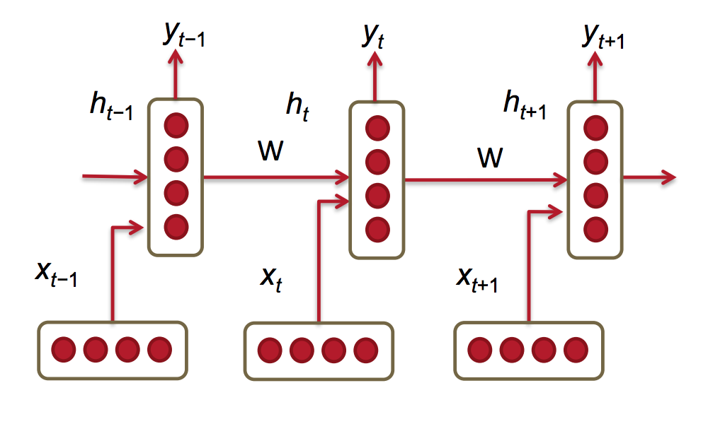
$$\begin{equation} \tag{Hidden State} h_t = \sigma(W_h h_{t-1} + W_x x_t) \end{equation}$$

$$\begin{equation} \tag{Prediction} \hat{y} = softmax(W_s h_t) \end{equation}$$

Suppose we wish to to give an RNN some text, in this case the lyrics to touching song, so that it can predict the next sequence of words, in this case so the RNN can keep giving us heartfelt lyrics. Using a vanilla RNN we would start off with a sequence of words represented as a sequence of vectors. Let’s say we have the sentence: “I love you for so many reasons, which means I love you for all seasons” (The Fuzz - I Love You For All Seasons). We would represent this as the sequence $X = {x_1,x_2,...x_n}$, where $x_1$ is a word vector representing “I”, $x_2$ is a word vector representing “love”, $x_t$ is the word at the $t$‘th time step.

We would give the first unit of the the RNN the word vector $x_1$, and some arbitrary initial past hidden state $h_0$ (usually just the zero vector). It would create $h_1$, a hidden representation the our current word sequence “I”. We could then use that hidden representation to predict the next word in our sequence, $\hat{y_1}$. We would pass $h_1$ to the second unit, and it would use the next word in the sequence $x_2$(“love”), to produce $h_2$, which is the hidden representation of our current word sequence “I love”. We could then use $h_2$ to predict the next word in our sequence $\hat{y_2}$. At any given time step $t$, our RNN will take the representation of our past sequence $h_{t-1}$, the current word $x_t$, and produce a hidden representation of our current sequence $h_t$, and can give us a prediction for the next word in our sequence $\hat{y_t}$.

Thus, by feeding our RNN some lyrics to a song, a sequence of words, it could continuously produce another predicted word, and take that as an input to itself to produce another word. With this continuous generation, we could end up with new sentences or paragraphs, or essays or maybe even a book if we let the RNN run long enough!

Since we process data in a sequential manner, representing our previous sequence as a hidden state vector $h_{t-1}$, the inductive bias encoded in this neural network architecture is that we can use what we have seen in the past determine what we might see in the future. This is further encoded in our matrices $W_h$ and $W_x$. Since we multiply $W_h$ with our past hidden state $h_{t-1}$, $W_h$ encodes what features of the past are important to determine the future. Since we multiply $W_x$ with our current word $x_t$, $W_x$ encodes what features of the present are important to determine the future.

This model has the right inductive biases for dealing with sequences and is thus successful, but it has very few parameters and thus has less flexibility than a model with more parameters. Moreover, Vanilla RNN’s have something called the vanishing/exploding gradient problem.

As time progresses the gradient of our loss functions tends to either zero, which means our model does not update during gradient descent and thus no learning occurs, or the gradient of our loss function explodes to such large numbers that we cannot compute, which also prevents us from updating our model. Let me give you some insight into why this occurs. If we have a loss function $E$, then we need compute the following gradient to update our model for time $T$:

$$\begin{equation} \frac{\partial E}{\partial W} = \sum_{t=1 }^{T }\frac{\partial E_t}{\partial W} \end{equation}$$

This total loss at time step $T$ requires us to sum our loss at each previous time step $t$. Now let’s expand the loss at each time step $t$: $$\begin{equation} \frac{\partial E_t}{\partial W} = \sum_{k=1 }^{t }\frac{\partial E_t}{\partial y_t} \frac{\partial y_t}{\partial h_t} \frac{\partial h_t} {\partial h_k} \frac{\partial h_k} {\partial W} \end{equation}$$

Let’s expand another crucial term: $$\begin{equation} \frac{\partial h_t} {\partial h_k} = \prod_{j=k+1}^{t} \frac{\partial h_j} {\partial h_{j-1}} \end{equation}$$

We have an upper-bound for $\frac{\partial h_j} {\partial h_{j-1}}$ given by the bounds of two matrix norms: $$\begin{equation} || \frac{\partial h_j} {\partial h_{j-1}} || \leq ||W^T|| ||diag[f\prime(h_{j-1}) ] || \leq \beta_W \beta_h \end{equation}$$

Thus we can say $$\begin{equation} || \frac{\partial h_t} {\partial h_k} || = || \prod_{j=k+1}^{t} \frac{\partial h_j} {\partial h_{j-1}} || \leq (\beta_W \beta_h)^{t-k} \end{equation}$$

If $\beta_W \beta_h$ is less than one, $(\beta_W \beta_h)^{t-k}$ and thus $\frac{\partial h_t} {\partial h_k}$ will tend towards zero, and if $(\beta_W \beta_h)$ is greater than one, than $(\beta_W \beta_h)^{t-k}$ and thus $\frac{\partial h_t} {\partial h_k}$ will tend towards and an incredibly large number that we can’t compute, and thus our total gradient: $$\begin{equation} \frac{\partial E}{\partial W} = \sum_{t=1 }^{T }\sum_{k=1 }^{t } \frac{\partial E_t}{\partial y_t} \frac{\partial y_t}{\partial h_t} (\prod_{j=k+1}^{t} \frac{\partial h_j} {\partial h_{j-1}}) \frac{\partial h_k} {\partial W} \end{equation}$$

will tend towards either zero or an uncomputable number.

Alas, fantastic folks have devised other great models that mitigate the vanishing gradient problem, while incorporating more inductive biases and flexibility into those models!

Gated Recurrent Unit (GRU)

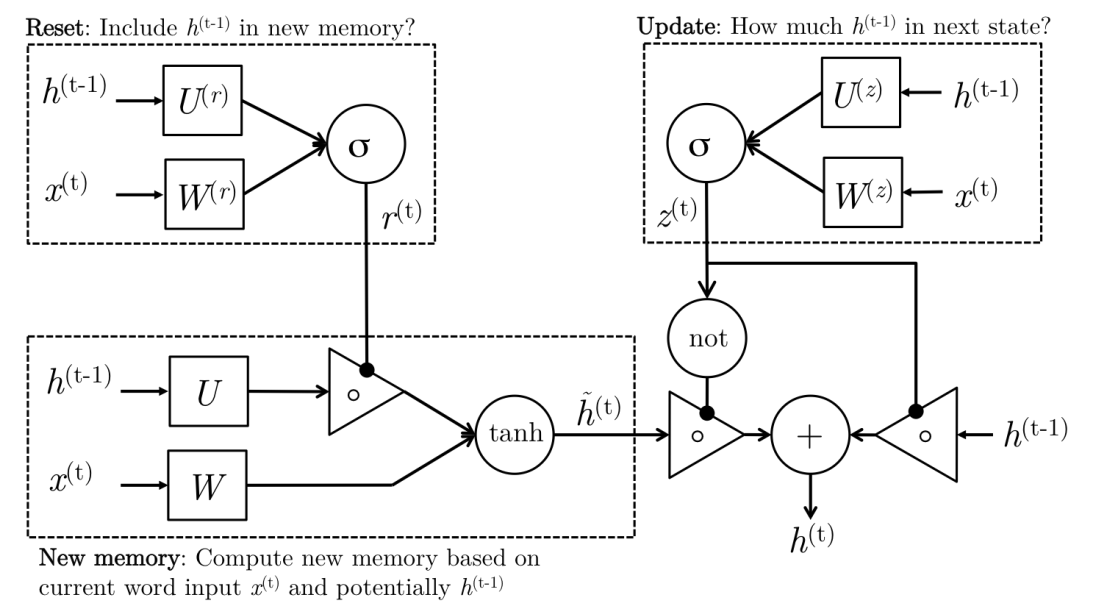
$$\begin{equation} \tag{Reset Gate} r_t = \sigma(W_r x_t + U_r h_{t-1}) \end{equation}$$

$$\begin{equation} \tag{New Memory } \tilde{h_t} = \tanh(r_t \odot U h_{t-1} + W x_t) \end{equation}$$

$$\begin{equation} \tag{Update Gate} z_t = \sigma(W_z x_t + U_z h_{t-1}) \end{equation}$$

$$\begin{equation} \tag{Hidden State} h_t = (1-z_t)\odot \tilde{h_t} + z_t \odot h_{t-1} \end{equation}$$

With GRU’s, we processes sequences of text in the same sequential manner, but the model has some extra parameters to it that help alleviate our vanishing gradient problem, all while encoding inductive biases we shall discuss!

Reset Gate:

The reset gate utilizes the current word in our sequence, with the hidden state representing our past sequence to determine how much to consider the past sequence in forming a new memory of our sequence.

New Memory:

New memory is formed by taking our current word in the sequence and determines its importance in the new memory with the $W$ matrix. It then utilizes the reset gate and the $U$ matrix to determine how important the past sequence is in forming a new memory. By explicitly utilizing including a reset gate and the the $U$ matrix, we have a more expressive model that is better able to utilize the important components of the past sequence while discarding irrelevant components.

Update Gate:

The update gate is utilized to determine how much our newly formed memory and our past sequence should contribute to representing our new sequence.

Hidden State:

Our new hidden state for our current sequence is computed by taking a weighted sum of the the newly formed memory, and our past sequence’s hidden state. These weights are determined by the update gate. Since the update gate is computed with a sigmoid function, our values are between zero and one. Thus $z_t$ and $1-z_t$ are between zero and one, and add up to one. Given these weights, when features of the previous hidden state are given importance in determining the new hidden state, those features in the newly formed memory are given less importance for determining the new hidden state.

Long Term Short Memory (LSTM)

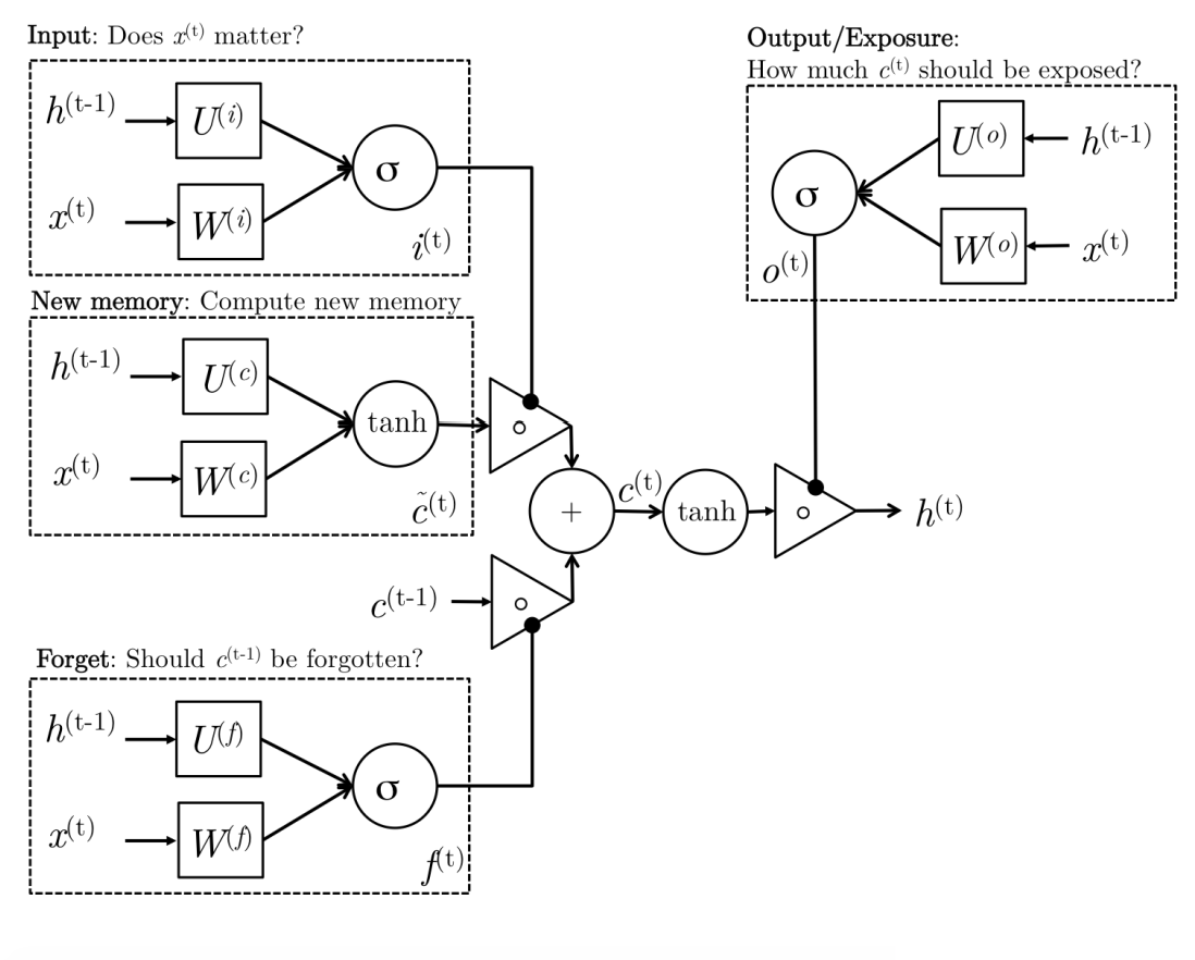
$$\begin{equation} \tag{ Input Gate} i_t = \sigma(W_i x_t + U_i h_{t-1}) \end{equation}$$

$$\begin{equation} \tag{Forget Gate } f_t = \sigma(W_f x_t + U_f h_{t-1}) \end{equation}$$

$$\begin{equation} \tag{Output Gate } o_t = \sigma(W_o x_t + U_o h_{t-1}) \end{equation}$$

$$\begin{equation} \tag{New Memory } \tilde{c_t} = \tanh(W_c x_t + U_c h_{t-1}) \end{equation}$$

$$\begin{equation} \tag{Final Memory} c_t = f_t \odot c_{t-1} + i_t \odot \tilde{c_t} \end{equation}$$

$$\begin{equation} \tag{Hidden State} h_t = o_t \odot \tanh(c_t) \end{equation}$$

Input Gate:

Uses the input word and past hidden state to determine how the new word in our sequence should influence our final new memory formation.

Forget Gate:

Determines how much the past memory should influence our new final memory formation. Can give us to completely forget what we learned before, or to continue to propagate our past memory!

New Memory:

We form a new memory utilizing our past hidden state representing our past sequence, and the new word we encountered in our sequence.

Final Memory:

For our final memory formation, we use the input gate to determine what’s important from our new memory, and the forget gate to determine what’s important from our past memory to form a final memory!

Output Gate:

Our finalized memory is rich in information, so the the output gate determines what aspects of this new memory are important for representing a new hidden state for our current sequence.

Hidden State:

The new hidden state new representation of our current sequence!